Logistic growth is one of the most fundamental models in ecology, biology, and population studies, providing a realistic framework for how a population grows over time when resources are limited. Unlike exponential growth, which assumes limitless resources and results in a perpetually increasing curve, logistic growth recognizes that every environment has a finite capacity to sustain life. This constraint introduces competition and ultimately slows the rate of increase, leading to a characteristic “S-shaped” curve.
The concept of logistic growth, formalized in the 19th century, is essential for predicting population dynamics, managing natural resources, and understanding everything from bacterial cultures in a petri dish to the global spread of new technologies.
1. The Principle of Logistic Growth
Logistic growth describes the change in population size ($N$) over time ($t$) when restricted by limiting factors. These factors—which can include food supply, water, nesting sites, or waste accumulation—determine the environment’s carrying Capacity.
Defining Carrying Capacity ($K$)The carrying Capacity ($K$) is the maximum population size that a specific environment can sustain indefinitely, given the available resources. It is the ceiling of the growth curve. As a population approaches $K$, resource competition intensifies, birth rates decline, and death rates rise, slowing growth.
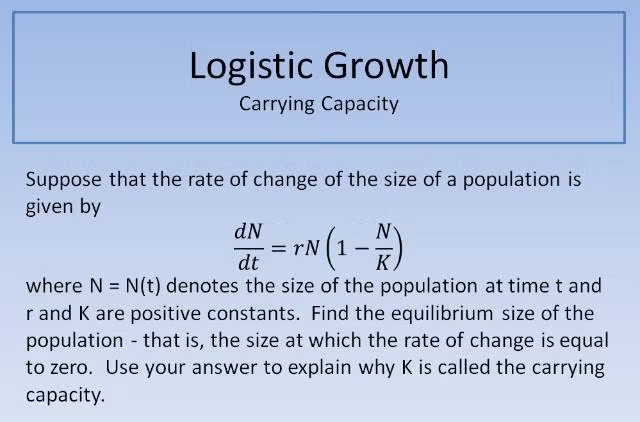
The mathematical formulation that describes this growth is:
\frac{dN}{dt} = r_{max} N \left(\frac{K-N}{K}\right)
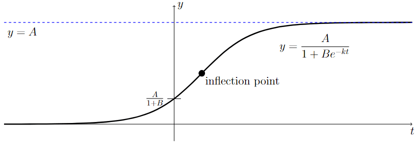
This equation models the change in population size per unit time (\frac{dN}{dt}). The characteristic result of this equation is a sigmoid or S-shaped curve that visually represents the three main phases of growth.
2. Key Components of the Logistic Equation
To fully grasp the dynamics of the logistic model, we must define its core variables:
\mathbf{\frac{dN}{dt}} (Population Growth Rate): The rate of change in the number of individuals over time. This value is highest when the population is halfway to the carrying capacity (N = K/2).
\mathbf{r_{max}} (Maximum Per Capita Growth Rate): This is the intrinsic rate of growth, representing the rate at which the population would grow if resources were unlimited (as in the exponential model).
\mathbf{N} (Population Size): The current number of individuals in the population.
\mathbf{K} (Carrying Capacity): The maximum sustainable population size of the environment.
The term \left(\frac{K-N}{K}\right) is the most essential element, as it introduces density dependence. As the current population (N) approaches the carrying capacity (K), the value of this fraction approaches zero, causing the overall growth rate (\frac{dN}{dt}) to approach zero.
3. Stages of the S-Shaped Curve
The logistic growth curve is composed of three distinct phases:
A. Lag Phase
When the population size (N) is tiny, the growth is initially slow. Individuals are establishing themselves, and the population is small, resulting in a low reproductive rate.
B. Exponential (or Logarithmic) Phase
As N increases and is still much smaller than K (i.e., N \ll K$), the term \left(\frac{K-N}{K}\right) is close to 1. In this phase, the population grows nearly exponentially because resources are abundant and limiting factors are minimal. The growth rate (\frac{dN}{dt}) reaches its maximum speed at the inflection point (N=K/2).
C. Stationary (or Plateau) Phase
As N approaches K, the term \left(\frac{K-N}{K}\right) approaches zero. The population growth rate slows drastically, and the size oscillates around $K$. At this point, the birth rate equals the death rate, resulting in zero population growth.
4. Logistic vs. Exponential Growth
The distinction between logistic and exponential (or Malthusian) growth models is critical for ecological accuracy.
| Feature | Exponential Growth | Logistic Growth |
| Growth Pattern | J-shaped curve | S-shaped (sigmoid) curve |
| Resource Assumption | Unlimited resources | Limited resources |
| Limiting Factors | Absent or negligible | Density-dependent factors (e.g., competition) |
| Applicability | Short-term growth under ideal conditions | Long-term growth under natural, constrained conditions |
| Final State | Theoretical infinite growth | Plateau at carrying capacity ($K$) |
While exponential growth may accurately describe a population’s initial burst in a new, unexploited environment, the logistic model offers a more accurate long-term view because, in reality, no biological population can grow indefinitely.
5. Applications Beyond Biology
While rooted in ecology, the logistic model has proven to be a robust predictive tool in many non-biological fields:
- Technology Adoption: The adoption rate of new technologies (e.g., smartphones, social media platforms) often follows an S-curve. Initial slow adoption (early adopters), followed by rapid growth (mass market), and finally, a plateau as the market becomes saturated.
- Economics: It can model the diffusion of products through a market, showing how sales rise quickly after initial market entry and then level off once all potential customers have been reached.
- Epidemiology: The initial phase of an infectious disease outbreak (before major countermeasures) can often resemble exponential growth, but the total number of infected individuals follows a logistic curve, leveling off as the susceptible population diminishes.
In summary, logistic growth is a powerful concept that goes beyond simple multiplication, incorporating real-world constraints. Acknowledging the limits imposed by carrying Capacity provides a realistic, predictive model of growth in diverse, dynamic systems.